Scaling using logarithms, linearizing data with logs + interpreting: notes and practice questions

The following table shows the number of days, $d$, since a new mobile application was launched and the percentage of its initial active user base, $x$, remaining at the beginning of that day.

The following table shows the natural logarithm of both $d$ and $x$ on these days, rounded to 2 decimal places.

Use the data in the second table to find the value of $m$ and the value of $b$ for the regression line, $\ln x = m(\ln d) + b$.

Assuming that the model found in part (a) remains valid, estimate the percentage of active users remaining when $d = 25$.

A biologist is studying the growth of a certain bacterial population, $N$, over time, $T$ (in hours). She created a scatter plot with $T$ on the x-axis and $\log_{10}N$ on the y-axis.

The biologist noticed that the points had a strong linear correlation, so she drew a line of best fit, as shown in the diagram. The line passes through the points $(0, -0.8)$ and $(5, 12.7)$.

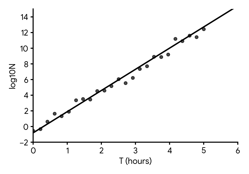
Find an equation for $N$ in terms of $T$.

The biologist also investigates the relationship between the population size, $N$, and the nutrient level, $S$. She believes that the data can be modelled by $N = c\sqrt{S} + d$, where $c$ and $d$ are constants, and she decides to create a scatter plot to verify her belief.

State what expression the biologist should plot on each axis to verify her belief.

The scatter plot from part (b) has a linear relationship, and the biologist finds $c = 3.5$ and $d = 8.2$.

Find an equation for $T$ in terms of $S$.

(a) The growth of a bacterial colony's area, $A$, over time, $t$, is being studied under specific conditions. The area $A$ is measured in square micrometers ($\mu m^2$) at the end of each hour $t$ for five consecutive hours. The data is recorded in Table 1.

**Table 1: Time $t$ (hours) and Area $A$ ($\mu m^2$)**

It is believed that the growth of the colony can be modelled by an equation of the form $A = k \times t^p$.

Use power regression on your graphic display calculator to find the value of $k$ and the value of $p$. Give your answers to three significant figures.

(b) The values of $t$ and $A$ can be transformed such that $x = \ln t$ and $y = \ln A$. Table 2 shows data for $x$ and $y$ to three decimal places.

**Table 2: Transformed data $x = \ln t$ and $y = \ln A$**

Find the linear regression equation of $y$ on $x$, in the form $y = cx + d$. Give the values of $c$ and $d$ to three decimal places.

(c) Hence, show that this linear regression is equivalent to the power regression found in part (a).

A school administrator is tracking the spread of a rumour among students. The number of students, $S$, who have heard the rumour is recorded $t$ hours after it began. The first results obtained are shown in the top two rows of the table below.

Complete the last row of the table, giving your answers to three decimal places.

Draw a graph of $\log_{10} S$ against $t$, using appropriate scales on the axes.

Hence, state the type of model that best fits the data displayed in part (b).

The school counsellor suggests that the number of students who have heard the rumour can be modelled by $S(t) = A \times B^t$.

Explain why the school counsellor is correct.

Hence, determine the values of the parameters $A$ and $B$ of the school counsellor's model, showing all your calculations. Give your answers to three significant figures.

The intensity of sound, $I$ (in W/m$^2$), from a point source varies inversely as the square of the distance, $r$ (in metres), from the source.

When $r = 10$ m, the intensity $I = 0.005$ W/m$^2$.

Find an equation for $I$ in terms of $r$.

Find the value of $I$ when $r = 25$ m.

Identify which two of the following graphs would form a straight line.

A. $I$ against $r$

B. $I$ against $r^2$

C. $I$ against $r^{-2}$

D. $\log_{10}I$ against $\log_{10}r$

E. $\log_{10}I$ against $r$

F. $I$ against $\log_{10}r$

For each of these two graphs identified in part (b.i), find the value of the gradient of the line formed.

A cup of hot tea is placed in a room with a constant ambient temperature of 22°C. The temperature of the tea, $T$ in degrees Celsius, is recorded at various times, $t$ in minutes.

It is assumed that the temperature difference, $D = T - 22$, follows an exponential decay model. To linearize the data, a graph of $\text{ln}(D)$ is plotted against $t$. This graph is a straight line that passes through the points $(4, 3.8)$ and $(12, 2.2)$.

(a) Find the equation of the straight line in the form $\text{ln}(D) = mt + c$, where $m$ and $c$ are constants.

(b) Hence,

(i) find an expression for $D$ in terms of $t$, writing your answer in the form $D = Ae^{kt}$.

(ii) calculate the temperature of the tea, $T$, when $t = 20$ minutes.