Phase portrait (for solutions to coupled systems) & sketching trajectories: notes and practice questions
- Coupled differential equations: System where rates of change of variables depend on each other, typically linear in matrix form .
- Phase portrait: Diagram illustrating how and values change over time, displaying typical solution trajectories.
- Solution trajectory: Specific path on a phase portrait based on initial conditions.
- Equilibrium point: Coordinate where and .
- Stability of the origin: Depends on the eigenvalues of the matrix .
- Matrix form of coupled differential equations:
- Exact solution formula (HL): For real, distinct eigenvalues with eigenvectors :
where are constants found using initial conditions.
- Second order differential equation conversion (HL): For , substitute .
- Resulting coupled system: and .
- Corresponding matrix: .
- Finding an equilibrium point: Set and , then solve the resulting equations simultaneously for .
- Determining phase portrait shape (HL, based on eigenvalues of ):
- Both real, one positive, one negative: Saddle point; trajectories approach along negative eigenvector, curve away along positive.
- Both real and negative: All trajectories converge to origin, curving towards the eigenvector of the least negative eigenvalue.
- Purely imaginary: Circular or elliptical orbits around the origin (unstable).
- Complex with a positive real part: Trajectories spiral away from the origin (unstable).
- Complex with a negative real part: Trajectories spiral in towards the origin (stable).
- Determining direction of spirals/orbits (HL):
- Choose a simple point (e.g., or ).
- Substitute its coordinates into and to find the initial velocity vector.
- Interpret the vector's direction to determine clockwise or anticlockwise motion.
- Sketching a specific solution trajectory (HL):
- Mark the initial point.
- Determine the initial direction by substituting the initial into and .
- Draw a continuous curve from the initial point, following the initial direction and conforming to the overall phase portrait shape.
- GDC use: Use simultaneous equation solver to find constants and from initial conditions.
- HL distinction: Coupled differential equations and phase portraits are exclusively HL topics (Topic 5.7).
- Contextual interpretation: In a converted second-order system where , the -axis represents velocity.
- Saddle point: Term for the origin when eigenvalues are real with opposite signs.
- Exact solution formula limits: Applicable only when eigenvalues of are real and distinct.
How it is examined
A question gives the coefficient matrix, asks for the eigenvalues (AHL 1.15 machinery again), and then asks what kind of equilibrium the origin is and how trajectories behave near it, sketch included. The restriction to distinct, non-zero eigenvalues means a student never has to handle the repeated or zero-eigenvalue edge cases, and the qualitative classification table above is worth memorising rather than re-deriving under time pressure.
The eigenvalue classification above.
- Sketch the phase portrait for solutions of coupled differential equations of the form , .
- Carry out a qualitative analysis of future paths for distinct real, complex and imaginary eigenvalues.
- Sketch trajectories and use phase portraits to identify equilibrium points, stable populations and saddle points.
Linking questions
- Other contexts: the Jacobian matrix, used to investigate the stability of equilibrium states for non-linear differential equations.
Practice questions
6 questions · 4 medium · 2 hardQuestion 1
MediumPaper 1 · calculator14 marksThe populations of two interacting species, A and B, in a controlled environment are modelled by the following system of linear differential equations:
where represents the population of species A and represents the population of species B at time . Find the general solution for this system.
Sketch the phase portrait for the system, clearly indicating the critical point, the equations of any asymptotes, and the general direction of trajectories. Briefly describe the long-term behaviour of the populations.
Start by writing the system in matrix form . Then, find the eigenvalues and corresponding eigenvectors of the matrix . The general solution will be a linear combination of these exponential solutions.
The critical point is at the origin. The type of critical point is determined by the eigenvalues (real and opposite signs indicate a saddle point). The asymptotes are given by the lines corresponding to the eigenvectors. Remember to show the direction of flow based on the sign of the eigenvalues: positive eigenvalues mean trajectories move away, negative eigenvalues mean trajectories move towards the origin.
Question 2
HardPaper 2 · calculator22 marksThe concentration of a chemical, (in mol dm), in a reaction vessel at time seconds is modelled by the differential equation
(a) (i) Use the substitution to show that this equation can be written as
.
(ii) Find the eigenvalues for the matrix .
(iii) Hence state the long-term rate of change of the chemical concentration.
The chemical reaction is now subjected to an external input, and the equation for the concentration is amended to
.
(b) (i) Use the substitution to write the differential equation as a system of coupled, first order differential equations. State the initial conditions given that, at , the concentration of chemical C is mol dm and its rate of change is mol dm s.
(ii) Use Euler's method with a step length of to find the concentration of the chemical when s. Give your answer to three significant figures.
(iii) Find the long-term rate of change of the chemical concentration.
Substitute and into the given second-order differential equation. Then, express both and in terms of and to form the matrix equation.
To find the eigenvalues of a matrix , solve the characteristic equation , where is the identity matrix.
Consider the sign of the eigenvalues. What does this imply about the stability of the system and the behavior of and as ?
Similar to part (a.i), but now include the non-homogeneous term in the equation for . Don't forget to state the initial values for and .
Set up the recurrence relations for and using Euler's method. You will need to perform 10 iterations to reach from . Keep track of , , and at each step.
For a non-homogeneous second-order ODE with a constant forcing term, the long-term solution (particular solution) will be a polynomial of the same degree as the forcing term. In this case, since the forcing term is , assume a particular solution of the form . Then, find .
Question 3
MediumPaper 2 · calculator20 marksA population model for two interacting species, and , is described by the following system of coupled differential equations, where and represent the deviations from their equilibrium populations. (a) Determine (with a worked reason) whether the populations of both species tend towards their equilibrium, move away from their equilibrium, or exhibit another behaviour.
(b) Determine (with a worked reason) whether the populations of both species tend towards their equilibrium, move away from their equilibrium, or exhibit another behaviour.
(c) Determine (with a worked reason) whether the populations of both species tend towards their equilibrium, move away from their equilibrium, or exhibit another behaviour.
(d) Determine (with a worked reason) whether the populations of both species tend towards their equilibrium, move away from their equilibrium, or exhibit another behaviour.
To determine the behaviour of solutions near the equilibrium, form the coefficient matrix and find its eigenvalues. The sign of the real parts of the eigenvalues will indicate whether solutions move towards or away from the origin.
Remember that if the eigenvalues have opposite signs, the equilibrium point is a saddle point, meaning solutions move away from the origin.
When eigenvalues are complex, the behaviour involves spirals. The sign of the real part of the complex eigenvalues determines if the spirals move towards or away from the origin.
If the eigenvalues are purely imaginary, the solutions will orbit the equilibrium point without moving towards or away from it.
Question 4
HardPaper 3 · calculator31 marksThe following question explores a possible method of drawing phase portraits for non-linear coupled systems, taking a predator-prey model as a particular example.
A forest ecosystem contains a population of rabbits (, measured in hundreds), and a population of wolves (, measured in hundreds).
Research indicates that the population dynamics of both rabbits and wolves can be modelled by the following differential equations, in which is measured in years.
for
At a specific time, there are 400 rabbits and 400 wolves, represented here by the coordinate pair (4, 4). At this time, determine the rate of change of
rabbits.
wolves.
There are two equilibrium points for the populations: A(0, 0) and B ().
Explain why A is an equilibrium point.
Find the value of and the value of .
At points close to A(0, 0), we can ignore the terms, so that the system can be approximated by:
for .
By solving these two differential equations,
find an expression for in terms of .
find an expression for in terms of .
Using your answers from part (c), show that phase portrait trajectories close to A may be given by the equation , where is a positive constant.
Hence sketch, on a phase portrait, one possible trajectory for small values of and .
Now consider points close to B on the phase plane. These coordinates can be rewritten as and , where and are the values from part (b)(ii).
By substituting into the original model, show that, for small values of and :
Similarly, it can be shown that .
Given that , where is a square matrix, write down .
By finding the eigenvalues of , describe the path of the trajectories close to point B.
Hence sketch a complete set of trajectories in the phase plane for the original model, clearly indicating both equilibrium points.
In this forest ecosystem, at a specific time, there are 400 rabbits and 400 wolves.
Based on the values found in part (a), the wildlife keeper is worried and assumes that the wolves will quickly die out. Suggest whether this assumption is supported by the model. Justify your answer.
Substitute the given population values for and into the differential equation for . Remember that and are measured in hundreds.
Substitute the given population values for and into the differential equation for .
An equilibrium point is where the populations do not change. Consider what this means for the rates of change and .
At an equilibrium point, both and . Set both differential equations to zero and solve the resulting system of algebraic equations.
These are separable differential equations. Separate the variables and integrate both sides. Remember to include the constant of integration.
Similar to part (c.i), solve the differential equation for .
To eliminate , raise to a power and to a power such that the exponents of become additive inverses (e.g., and ). Then multiply the resulting expressions.
The equation describes the shape. Consider the signs of and near A(0,0) to determine the direction of the trajectory.
Substitute and into the original differential equation for . Expand the terms and cancel out constants, then identify and ignore the higher-order terms (like ) for small and .
The coefficients of and in the linearised equations for and form the entries of the matrix .
To find the eigenvalues, solve the characteristic equation , where is the identity matrix. The nature of the eigenvalues (real, complex, purely imaginary) determines the type of equilibrium point.
Combine the information from parts (d.ii) and (g). A(0,0) is a saddle point, and B(5,6) is a center. Remember to indicate the direction of trajectories and ensure they remain in the first quadrant.
Refer to your sketch in part (h). Consider where the initial point (4,4) might lie relative to the equilibrium point B, and what the trajectories around B represent.
Question 5
MediumPaper 1 · calculator6 marksThe populations of two interacting bacterial strains, Alpha and Beta, in a controlled environment are modelled by a system of coupled differential equations. Let be the population of strain Alpha (in thousands) and be the population of strain Beta (in thousands).
The system is given by:
At time hours, the population of strain Alpha is thousand and the population of strain Beta is thousand.
Find the value of at .
The eigenvalues for this system are .
On the following phase portrait, sketch the trajectory that passes through the point . Clearly indicate the direction of this trajectory.
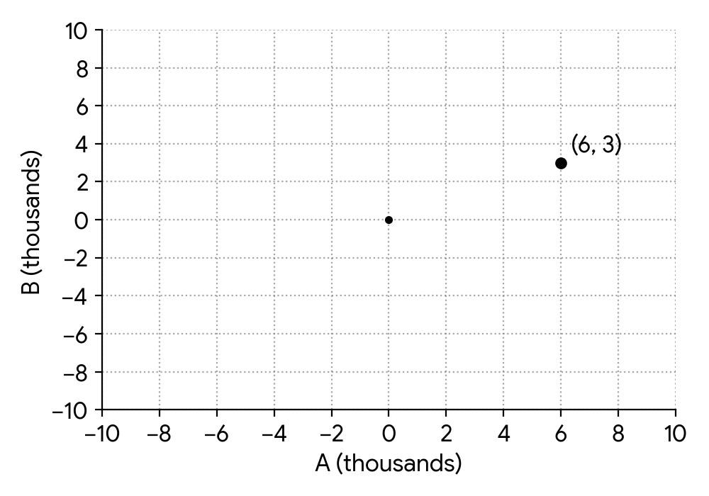
To find , you need to calculate and at the given initial conditions. Remember the chain rule for derivatives: .
Eigenvalues of the form (where is a real number and ) indicate a center at the origin, meaning the trajectories are closed loops (ellipses or circles) around the origin. To determine the direction, evaluate the signs of and at the given point .
Question 6
MediumPaper 2 · calculator15 marksA microscopic particle is observed moving in a fluid. Its position metres, relative to a fixed origin O, at time seconds (), is modelled by the system of differential equations:
Find the eigenvalues of the matrix , giving your answers in the form , where .
State what indicates about the path of the particle.
State what the sign of indicates about the path of the particle.
At time , the particle is at position .
At time , find the value of .
Find the value of at time .
Use your answers to parts (b) and (c) to sketch the path of the particle.
To find the eigenvalues of a matrix , you need to solve the characteristic equation , where is the identity matrix and represents the eigenvalues.
Consider the general behaviour of solutions to systems of differential equations when the real part of the eigenvalues is non-zero.
A negative real part of the eigenvalues indicates a stable node or spiral, while a positive real part indicates an unstable node or spiral.
Substitute the initial position into the given differential equation for .
Remember that . You will need to calculate first.
Consider the starting point, whether the path spirals inwards or outwards, and the initial direction of movement indicated by .
No question on this page matches those filters. Try another difficulty or paper.
Every Phase portrait (for solutions to coupled systems) & sketching trajectories question, marked for you
Every answer is marked mark by mark, IB-style, and the AI tutor helps when you are stuck.
Where marks are lost
- Using your own wrong value after failing a "show that." All follow through is withdrawn for the rest of that question.
- Leaving an answer in calculator notation. Never accepted in a final answer, and AI's constant calculator use makes this the easiest slip in the whole subject.