Spearman’s rank (+ limitations of pearson / spearman): notes and practice questions
- Spearman's Rank Correlation Coefficient () measures the strength and direction of a monotonic relationship between two variables.
- A monotonic function either only increases or only decreases.
- values range from -1 to 1:
- Closer to 1 or -1 indicates a stronger monotonic correlation of rankings.
- 1: strong positive monotonic relationship.
- -1: strong negative monotonic relationship.
- Pearson's PMCC () tests for a linear relationship and is highly sensitive to outliers.
- Spearman's Rank () tests for a monotonic relationship and is generally not affected by outliers as it uses ranks.
- To calculate :
- Rank all x-values (e.g., 1 for highest, n for lowest).
- Rank all y-values independently, using the same ranking rule as x.
- For tied values, assign the average of the ranks they would normally occupy (e.g., 3rd, 4th, 5th tied values all get rank ).
- Use a GDC to find the standard Pearson's PMCC of these newly created lists of ranks; this result is .
- Use a GDC to plot a scatter diagram of raw data to visually assess linearity or monotonicity.
- When interpreting coefficients:
- High suggests a strong positive/negative linear correlation.
- High suggests a strong positive/negative monotonic correlation, which is not necessarily linear.
- If is noticeably closer to 1 or -1 than , a non-linear monotonic model may better describe the relationship.
- The calculation and interpretation of are identical for IB AI SL and HL.
How it is examined
Distinctive to AI. The reliable question is a comparison: compute both coefficients, then say which is more appropriate for this data and why, with outliers or non-linearity as the reason. Averaging tied ranks is a stated rule and a common slip. Do not ask for a derivation.
- Spearman's rank correlation coefficient, .
- Awareness of the appropriateness and limitations of Pearson's product-moment correlation coefficient and of Spearman's rank correlation coefficient, and the effect of outliers on each.
Not required: derivation or proof of Pearson's product-moment correlation coefficient and Spearman's rank correlation coefficient.
Linking questions
- Links to other subjects: fieldwork (biology, psychology, environmental systems and societies, sports exercise and health science).
- Aim 8: Frank Oppenheimer wrote "Prediction is dependent only on the assumption that observed patterns will be repeated". That is the danger of extrapolation, and there are many examples of its failure, for example share prices, the spread of disease, climate change.
- TOK: does correlation imply causation? Given that a set of data may be approximately fitted by a range of curves, where would a mathematician seek knowledge of which equation is the "true" model?
- Links to websites: www.wikihow.com/Calculate-Spearman%27s-Rank-Correlation-Coefficient
- External website: use of databases such as Gapminder.
Practice questions
14 questions · 12 medium · 2 hardQuestion 1
MediumPaper 1 · calculator6 marksDr. Anya Sharma, a university researcher, is investigating the belief that students who spend more time studying tend to achieve higher exam scores. She randomly selects eight students and collects data on their average weekly study hours and their final exam scores.
Her data is shown in Table 1.
Table 1
Student | S1 | S2 | S3 | S4 | S5 | S6 | S7 | S8
---|---|---|---|---|---|---|---
Average weekly study hours | 10 | 15 | 5 | 20 | 12 | 8 | 25 | 18
Final exam score (out of 100) | 70 | 60 | 55 | 90 | 80 | 65 | 95 | 75
Dr. Sharma decides to calculate the Spearman's rank correlation coefficient.
Complete the table of ranks shown in Table 2, assigning rank 1 to the highest value.
Table 2
Student | S1 | S2 | S3 | S4 | S5 | S6 | S7 | S8
---|---|---|---|---|---|---|---
Rank – Study Hours | 6 | 4 | 8 | 2 | 5 | 7 | 1 | 3
Rank – Exam Scores | | | | | | | |
Calculate the value of , Spearman's rank correlation coefficient.
Dr. Sharma believes that students with a higher number of weekly study hours achieve higher exam scores. She carries out a hypothesis test using a 10% significance level with the following null hypothesis:
: In the population, there is no monotonic relationship between the number of weekly study hours and final exam scores.
Write down Dr. Anya Sharma's alternative hypothesis.
The critical value of for this test is 0.643.
State the conclusion of the hypothesis test, giving a reason.
Assign rank 1 to the highest value, rank 2 to the second highest, and so on, for the 'Exam Scores' row.
First, calculate the differences in ranks () for each student. Then, square these differences () and sum them up (). Finally, use the formula , where is the number of data pairs.
Consider the direction of the relationship Dr. Sharma is investigating (higher study hours leading to higher scores).
Compare your calculated from part (b) with the given critical value . If , you reject . Otherwise, you fail to reject . Remember to state your conclusion in context.
Question 2
HardPaper 2 · calculator21 marksDr. Anya Sharma, a sports scientist, is investigating the relationship between training habits and performance in junior athletes. She wants to collect data on the weekly training hours of junior swimmers. She decides to interview every 5th swimmer entering the training facility until she has a sample of 50 swimmers.
State the sampling method Dr. Sharma has used.
Dr. Sharma constructed the following box and whisker diagram to show the weekly training hours (in hours) of a sample of junior swimmers.
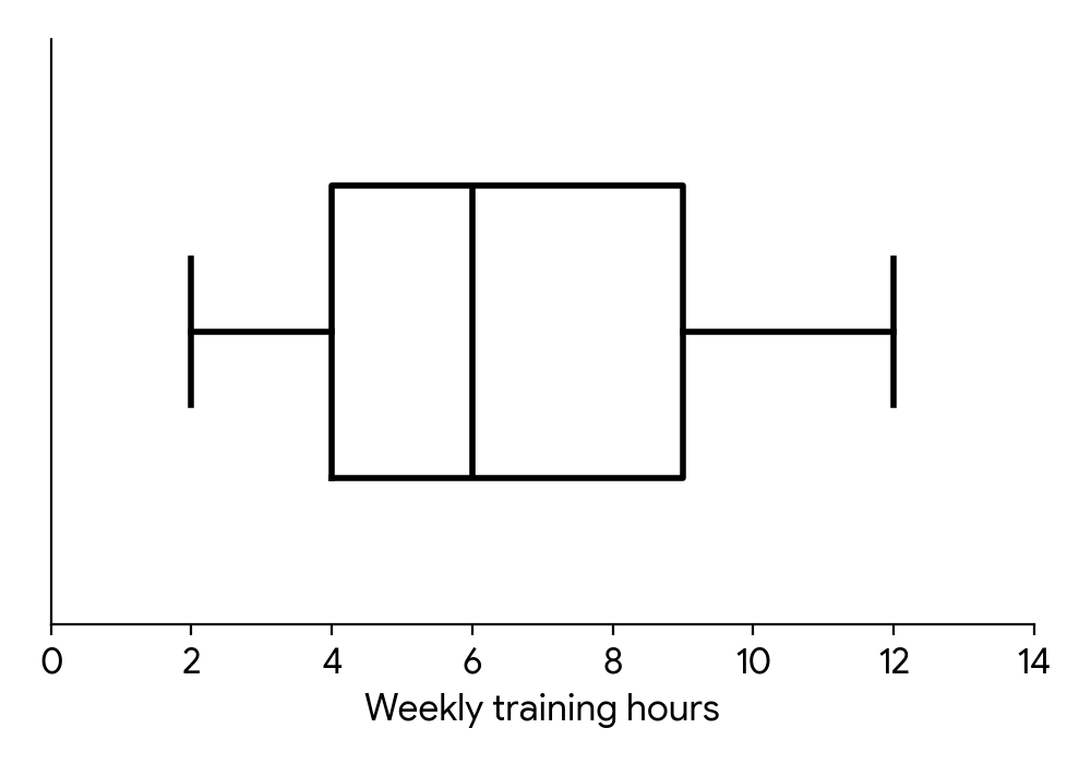
Write down the median weekly training hours.
Calculate the interquartile range for the weekly training hours.
One swimmer in the sample reported training for 15 hours per week. Dr. Sharma believes this swimmer's training time is not an outlier.
Determine whether Dr. Sharma is correct. Support your reasoning.
Dr. Sharma also collected data on the average weekly training hours () and the competition score () for a group of athletes. These data are represented on the scatter diagram.
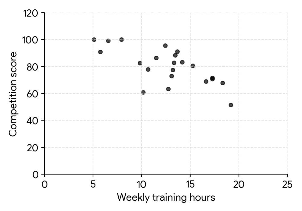
Describe the correlation between weekly training hours and competition score.
Dr. Sharma correctly calculates the equation of the regression line on for these athletes to be . She uses the equation to estimate the competition score for an athlete who trains 3 hours per week.
Find the competition score calculated by Dr. Sharma.
State whether it is valid to use the regression line on for Dr. Sharma's estimate in part (f). Give a reason for your answer, assuming the original data for training hours ranged from 5 to 20 hours.
Dr. Sharma investigated the relationship between an athlete's national competition rank and their average daily protein intake (in grams). She collected data for eight athletes, as shown in the table.
| Athlete | A | B | C | D | E | F | G | H |
|---|---|---|---|---|---|---|---|---|
| Competition Rank () | 1 | 2 | 3 | 4 | 5 | 6 | 7 | 8 |
| Protein Intake (g) () | 180 | 150 | 200 | 160 | 140 | 190 | 170 | 130 |
Dr. Sharma intends to analyse the data using Spearman's rank correlation coefficient, .
Copy and complete the information in the following table.
| Athlete | A | B | C | D | E | F | G | H |
|---|---|---|---|---|---|---|---|---|
| Rank - Competition Rank | 1 | |||||||
| Rank - Protein Intake |
Calculate the value of .
Interpret your result.
Consider how the sample is selected. Is there a systematic rule applied, or is it based on categories and targets?
The median is represented by the line inside the box of a box and whisker diagram.
The interquartile range (IQR) is the difference between the third quartile (Q3) and the first quartile (Q1).
An outlier is typically defined as a data point that falls more than 1.5 times the interquartile range (IQR) below the first quartile (Q1) or above the third quartile (Q3). Calculate the upper and lower fences.
Observe the general trend of the points on the scatter diagram. Do they tend to go up or down from left to right?
Substitute the given value of into the regression equation to find the corresponding value.
Consider if the value used for prediction falls within the range of the original data used to create the regression line.
Assign ranks to the 'Protein Intake' values. If 'Competition Rank' is already ranked from 1 to 8 (best to worst), then for 'Protein Intake', assign rank 1 to the highest intake, rank 2 to the next highest, and so on.
Use the formula for Spearman's rank correlation coefficient: , where is the difference between the ranks and is the number of data pairs.
Consider the sign and magnitude of . What does a positive or negative value mean, and what does a value close to 0 or 1 (or -1) indicate about the strength of the relationship?
Question 3
MediumPaper 1 · calculator6 marksMs. Chen, a small business owner, wants to investigate if there is a monotonic relationship between the monthly advertising budget and the number of units of a new product sold. She collects data for eight months, as shown in Table 1.
Table 1: Monthly Advertising Budget and Units Sold
| Month | Advertising Budget (in $100s) | Units Sold |
|---|---|---|
| 1 | 2.5 | 120 |
| 2 | 3.0 | 150 |
| 3 | 1.8 | 95 |
| 4 | 4.2 | 170 |
| 5 | 3.5 | 110 |
| 6 | 2.0 | 180 |
| 7 | 4.8 | 230 |
| 8 | 3.2 | 130 |
Ms. Chen decides to calculate the Spearman's rank correlation coefficient. Complete the table of ranks shown in Table 2.
Table 2: Ranks for Advertising Budget and Units Sold
| Month | Rank of Advertising Budget () | Rank of Units Sold () |
|---|---|---|
| 1 | 3 | 3 |
| 2 | 5 | |
| 3 | 1 | 1 |
| 4 | 7 | |
| 5 | 2 | |
| 6 | 2 | |
| 7 | 8 | 8 |
| 8 | 4 |
Calculate the value of , Spearman's rank correlation coefficient.
Ms. Chen believes that a higher advertising budget leads to more units sold. She carries out a hypothesis test using a 10% significance level with the following null hypothesis:
: In the population, there is no monotonic relationship between the monthly advertising budget and the number of units sold.
Write down Ms. Chen's alternative hypothesis.
The critical value of for this test is 0.643.
State the conclusion of the hypothesis test, giving a reason.
To rank the data, assign rank 1 to the smallest value, rank 2 to the next smallest, and so on. If there are tied values, assign the average of the ranks they would have occupied.
Recall the formula for Spearman's rank correlation coefficient: , where is the difference in ranks for each pair of data and is the number of data pairs.
The alternative hypothesis () should reflect Ms. Chen's belief and contradict the null hypothesis. Consider if it's a positive, negative, or non-directional relationship.
Compare your calculated value from part (b) with the given critical value . If , you reject . Otherwise, you do not reject . Remember to consider the direction of the test.
Question 4
HardPaper 3 · calculator28 marks(a) TechInnovate is considering collecting more data for their analysis.
(i) State one advantage of increasing the sample size.
(ii) State one disadvantage of increasing the sample size.
(b) The production manager at Plant Alpha recorded the time, in minutes, taken to produce a batch of electronic components for 10 randomly selected batches:
Find the value of for this sample from Plant Alpha.
(c) A manager claims that Plant Alpha's production times are more consistent than Plant Beta's. Given that the sample standard deviation () for Plant Beta's production times is minutes, make one criticism of this claim.
(d) TechInnovate wants to compare the mean production times of Plant Alpha and Plant Beta using a pooled t-test.
(i) State the condition regarding population variances required to use a pooled t-test.
(ii) Given that for Plant Beta, a sample of batches yielded a mean production time of minutes and a sample standard deviation of minutes, state whether TechInnovate should use a pooled t-test in this case. Justify your answer.
(e) TechInnovate believes Plant Alpha has a lower mean production time than Plant Beta.
(i) State appropriate null and alternative hypotheses for the pooled t-test.
(ii) Find the p-value.
(iii) Given that the test is carried out at the 5% significance level, state the appropriate conclusion in context. Justify your answer.
(f) The company also investigates the relationship between operator experience (in years) and the number of defective items produced per day. A sample of 8 operators yielded the following data:
| Operator Experience (years) | Number of Defective Items |
|---|---|
| 2 | 15 |
| 5 | 10 |
| 3 | 13 |
| 8 | 7 |
| 1 | 18 |
| 6 | 9 |
| 4 | 12 |
| 7 | 8 |
(i) Assuming all requirements are met, perform a test at the 5% significance level to determine if there is a linear correlation between operator experience and the number of defective items. State the hypotheses and justify your conclusion.
(ii) If the requirements for this test are not met, state an alternative test that could be used.
(g) For the data in (f.i), the equation of the least squares regression line of defective items () on operator experience () is . Give, in context, an interpretation of the gradient in this model.
(h) TechInnovate uses a baseline model to predict the number of defective items () for a batch based on its size (): . The "Quality Deviation" () for a batch is defined as . A positive Quality Deviation indicates better-than-expected quality.
(i) Show that for a batch of components from Plant Beta that produced defective items, the Quality Deviation is .
(ii) To compare quality control, samples of Quality Deviation scores were collected:
- Plant Alpha: , ,
- Plant Beta: , ,
Assuming that the appropriate requirements are met, use a pooled t-test at a 5% significance level to determine if the mean Quality Deviation is higher in Plant Alpha than in Plant Beta. Write down your null and alternative hypotheses and justify your conclusion.
(i) Using the results from parts (e) and (h.ii), explain how each plant could claim they are performing better than the other plant.
Think about how a larger sample relates to the overall population.
Consider the practical implications of collecting more data.
Use your GDC to calculate the sample standard deviation ( or ).
Consider the nature of sample statistics versus population parameters, especially when values are close.
Recall the assumption about variances for a pooled t-test.
Compare the sample standard deviations of Plant Alpha (from part b) and Plant Beta.
Remember to define your parameters and specify the direction of the alternative hypothesis.
Use your GDC to perform a two-sample t-test with pooled variance, then adjust for the one-tailed hypothesis.
Compare the p-value with the significance level and relate it back to the original claim about production times.
Calculate the Pearson product-moment correlation coefficient () and its associated p-value. Formulate hypotheses for population correlation ().
Consider non-parametric alternatives for correlation when assumptions for Pearson's are violated.
The gradient represents the change in the dependent variable for a one-unit change in the independent variable.
First, calculate the predicted number of defective items using the model. Then, apply the definition of Quality Deviation.
Formulate hypotheses for the population mean Quality Deviation. Perform a one-tailed pooled t-test using your GDC.
Review the conclusions of the two t-tests. One test might favor Plant Alpha, while the other might not show a significant difference, which Plant Beta could use to their advantage.
Question 5
MediumPaper 1 · calculator8 marksA fitness coach wanted to investigate if there was a relationship between the number of hours clients spent in a specific yoga class per week and their flexibility score (measured on a scale of 1 to 100). The data from clients is shown in the table below.
| Hours of Yoga (per week) | Flexibility Score |
|---|---|
Calculate Spearman's rank correlation coefficient () for this data.
Interpret the value of and comment on its validity.
First, assign ranks to the 'Hours of Yoga' and 'Flexibility Score' data separately. Remember to use average ranks for tied values. Then, calculate the differences in ranks (), square them (), and find the sum of . Finally, apply the Spearman's rank correlation coefficient formula: .
For interpretation, consider the strength and direction of the correlation based on the calculated value. For validity, think about what type of relationship Spearman's rank correlation coefficient measures and why it is appropriate (or not) for this type of data.
Question 6
MediumPaper 1 · calculator8 marksA health researcher is investigating the relationship between the number of hours individuals spend exercising per week and their average weekly stress level (rated on a scale of to , where is very high stress). The data for participants is shown below:
| Exercise (hours/week) () | Stress Level (1-10) () |
|---|---|
(a) Construct a table of ranks for this data.
(b) Calculate Spearman's rank correlation coefficient for this data.
(c) The researcher concludes that increased exercise leads to lower stress levels. Using your calculations, comment on whether or not the researcher's conclusion is supported by the data. Suggest what conclusions you are able to make from your calculations.
To construct the table of ranks, order the data for each variable (Exercise hours and Stress level) from smallest to largest. Assign ranks starting from for the smallest value. If there are tied values, assign them the average of the ranks they would have occupied.
Use the formula for Spearman's rank correlation coefficient: , where is the difference between the ranks for each pair of data, and is the number of data pairs.
Consider the value of Spearman's rank correlation coefficient. What does its sign and magnitude indicate about the relationship between the two variables? Remember that correlation does not imply causation.
Question 7
MediumPaper 1 · calculator6 marksA research team is investigating various relationships between pairs of variables in different scientific and social contexts. For each of the six observed phenomena, a scatter plot was generated to visualize the relationship between the two variables. Your task is to match each description of the scatter plot (A-F) to the most appropriate pair of Pearson's product-moment correlation coefficient (PMCC) and Spearman's rank correlation coefficient () values (1-6).
Scatter Plot Descriptions:
(A) The data points form a perfectly straight line with a positive gradient, indicating a direct linear relationship.
(B) The data points follow a clear, consistently increasing curve, but not a straight line. The increase becomes steeper at higher values.
(C) The data points are widely dispersed with no apparent pattern or trend.
(D) The data points form a perfectly straight line with a negative gradient, indicating an inverse linear relationship.
(E) The data points follow a clear, consistently decreasing curve, but not a straight line. The decrease becomes less steep at higher values.
(F) The data points show a general tendency to decrease as one variable increases, but there is considerable scatter around any potential trend line.
Correlation Coefficient Pairs:
1. PMCC ,
2. PMCC ,
3. PMCC ,
4. PMCC ,
5. PMCC ,
6. PMCC ,
Remember that Pearson's product-moment correlation coefficient (PMCC) measures the strength and direction of a linear relationship, while Spearman's rank correlation coefficient () measures the strength and direction of a monotonic relationship. A perfect monotonic relationship (always increasing or always decreasing) will result in , even if it's not linear.
Question 8
MediumPaper 1 · calculator10 marks(a) A human resources manager collected data on the 'Employee Rank' (an ordinal measure assigned by senior management) and the average 'Customer Satisfaction Rating' (on a scale of to ) for eight employees. The data is shown in the table below:
| Employee Rank () | ||||||||
|---|---|---|---|---|---|---|---|---|
| Customer Satisfaction Rating () |
Explain why it might not be appropriate to use the Pearson's product-moment correlation coefficient (PMCC) in this case.
(b) Calculate Spearman's rank correlation coefficient () for this data.
(c) Interpret the value of and comment on its validity.
Consider the nature of the 'Employee Rank' variable and the assumptions required for PMCC.
First, rank both sets of data. Then calculate the differences in ranks () and the sum of the squared differences (). Finally, apply the formula for Spearman's rank correlation coefficient.
Consider the strength and direction of the correlation based on the calculated value. For validity, think about the sample size and what correlation implies.
Question 9
MediumPaper 1 · calculator6 marksTwo music critics, Liam and Chloe, independently rank eight newly released albums from 'Album 1' to 'Album 8' based on their artistic merit.
The albums are labelled 1 to 8 and the critics' ranks are shown in the table.
| Album | Liam's Rank | Chloe's Rank |
|---|---|---|
| 1 | 1 | 2 |
| 2 | 2 | 1 |
| 3 | 3 | 4 |
| 4 | 4 | 3 |
| 5 | 5 | 5 |
| 6 | 6 | 7 |
| 7 | 7 | 8 |
| 8 | 8 | 6 |
(a) Write down the rank that Liam awards Album 3.
(b) Calculate Spearman's rank correlation coefficient for these data.
(c) Comment on your answer to part (b) in terms of the ranks awarded by Liam and Chloe.
Locate 'Album 3' in the table and find the corresponding rank given by Liam.
First, find the differences in ranks () for each album, then square these differences (). Finally, use the formula for Spearman's rank correlation coefficient: .
Consider what a Spearman's rank correlation coefficient close to 1, -1, or 0 indicates about the relationship between the two sets of ranks.
Question 10
MediumPaper 2 · calculator16 marksThe scores of eight students in a national mathematics competition and the number of hours they spent studying are shown in the following table.
| Student | Score (y) |
|---|---|
| A | 92 |
| B | 88 |
| C | 85 |
| D | 80 |
| E | 75 |
| F | 72 |
| G | 68 |
| H | 65 |
(a)(i) For this data, find the upper quartile.
(a)(ii) For this data, find the interquartile range.
(b) Determine if Student A's score is an outlier for this data. Justify your answer.
A researcher is investigating the relationship between students' mathematics competition scores and their study hours to determine whether study hours can reasonably be used to predict a student's score.
The study hours of the students are shown in the table.
| Student | Study Hours (x) | Score (y) |
|---|---|---|
| A | 40 | 92 |
| B | 35 | 88 |
| C | 20 | 85 |
| D | 30 | 80 |
| E | 15 | 75 |
| F | 25 | 72 |
| G | 10 | 68 |
| H | 10 | 65 |
The researcher finds that, for this data, the Pearson's product moment correlation coefficient is .
(c) State whether it would be appropriate for the researcher to use the equation of a regression line for on to predict a student's score. Justify your answer.
The researcher then decides to find the Spearman's rank correlation coefficient for this data, and creates a table of ranks (lowest value = rank 1).
| Student | Score Rank | Study Hours Rank |
|---|---|---|
| A | 8 | 8 |
| B | 7 | 7 |
| C | 6 | a |
| D | 5 | 6 |
| E | 4 | 3 |
| F | 3 | b |
| G | 2 | 1.5 |
| H | 1 | c |
(d)(i) Write down the value of:
a,
(d)(ii) Write down the value of:
b,
(d)(iii) Write down the value of:
c.
(e)(i) Find the value of the Spearman's rank correlation coefficient .
(e)(ii) Interpret the value obtained for .
(f) When calculating the ranks, the researcher incorrectly read Student A's score as 90. Explain why the value of the Spearman's rank correlation does not change despite this error.
First, ensure the scores are ordered from lowest to highest. Then, identify the position of the upper quartile () for an even number of data points.
You will need to find the lower quartile () first. Remember that the interquartile range is the difference between the upper and lower quartiles.
An outlier is typically defined as a data point that falls below or above . Use the values of , , and you found in part (a).
Consider what a Pearson's correlation coefficient of indicates about the strength of the linear relationship between the variables.
Rank the 'Study Hours' data from lowest to highest. If there are ties, assign the average of the ranks they would have occupied.
Rank the 'Study Hours' data from lowest to highest. If there are ties, assign the average of the ranks they would have occupied.
Rank the 'Study Hours' data from lowest to highest. If there are ties, assign the average of the ranks they would have occupied.
Use the formula , where is the difference in ranks and is the number of data pairs. You may also use your GDC.
Consider the range of possible values for (from -1 to 1) and what positive or negative values close to 1 or -1, or close to 0, signify.
Think about how ranks are assigned. If a value changes but still maintains its relative position (e.g., still the highest or lowest), how does that affect its rank?
Question 11
MediumPaper 2 · calculator19 marksA botanist is investigating the relationship between the concentration of a new liquid fertilizer and the average height of a particular plant species. They prepare seven different concentrations of the fertilizer and grow a sample of plants at each concentration, recording the average height after a specific period.
The data collected is shown in the table below:
| Fertilizer concentration ( g/L) | Average plant height ( cm) |
|---|---|
Write down the value of the Spearman's rank correlation coefficient, .
Find the Pearson's product-moment correlation coefficient, .
Use your value of to state which two of the following would best describe the correlation between fertilizer concentration and average plant height.
Positive Negative Strong Weak No correlation
The relationship between fertilizer concentration and average plant height can be modelled by the regression equation .
Write down the value of .
Write down the value of .
According to this model, state in context what the value of represents.
A botanist uses the regression equation to estimate the average height of a plant grown with a fertilizer concentration of g/L.
Find this estimated height.
State two reasons that the botanist might use to justify the validity of this estimate.
To investigate the effectiveness of different fertilizer brands, the botanist conducts an experiment. They grow two groups of plants, one using 'Bio-Grow' (Brand A) and another using 'RootBoost' (Brand B), both at a standard concentration. They take a random sample of seven plants from each group and record their average heights (in cm) after a month.
Brand A (Bio-Grow) heights:
Brand B (RootBoost) heights:
The botanist conducts a t-test, at the level of significance, to see if the mean plant height using Brand A is different from the mean plant height using Brand B. They assume the population variances are the same.
For this test, the null hypothesis is .
Write down the alternative hypothesis.
Find the -value for this test.
State the conclusion of the test. Justify your answer.
State one additional assumption the botanist has made about the distributions to conduct this test.
Use your GDC to calculate the Spearman's rank correlation coefficient. Ensure your data is entered correctly.
Use your GDC's statistical functions to find the Pearson's product-moment correlation coefficient for the given data.
Consider the sign and magnitude of the Pearson's correlation coefficient to determine the direction and strength of the relationship.
Use your GDC to perform linear regression (LinReg(ax+b) ) on the data. The value of is the gradient.
The value of is the y-intercept from the linear regression calculation on your GDC.
The value of is the y-intercept, which occurs when . Consider what means in this context.
Substitute the given fertilizer concentration into the regression equation using your calculated values of and .
Consider whether the estimation involves interpolation or extrapolation, and the strength of the correlation.
The alternative hypothesis states what the experiment aims to show if the null hypothesis is false. The question asks if the mean heights are 'different'.
Use your GDC's 2-sample t-test function. Remember to select 'pooled' for equal variances.
Compare the -value to the significance level (). If , reject the null hypothesis.
Besides equal variances, what other assumption is typically made about the population distributions for a t-test?
Question 12
MediumPaper 2 · calculator16 marksA consumer electronics magazine conducted a review of 10 new smart home devices. Each device was rated on two criteria: a "User Satisfaction Score" (out of 10, based on extensive user feedback) and an "Expert Review Score" (out of 5, by professional reviewers).
The data for the 10 devices is shown in the table below:
| Device | P1 | P2 | P3 | P4 | P5 | P6 | P7 | P8 | P9 | P10 |
|---|---|---|---|---|---|---|---|---|---|---|
| User Satisfaction Score () | 8.1 | 7.5 | 9.0 | 6.8 | 7.5 | 8.5 | 6.0 | 9.2 | 7.0 | 8.8 |
| Expert Review Score () | 4.0 | 3.5 | 4.5 | 3.0 | 3.8 | 4.2 | 2.5 | 4.8 | 3.2 | 4.0 |
(a) For the User Satisfaction Score (),
(i) find the upper quartile.
(ii) find the interquartile range.
(b) Show that the highest User Satisfaction Score is not an outlier for this data.
The scores for both criteria were ranked to calculate Spearman's rank correlation coefficient, . The ranks for the Expert Review Score () are shown in the following table:
| Device | P1 | P2 | P3 | P4 | P5 | P6 | P7 | P8 | P9 | P10 |
|---|---|---|---|---|---|---|---|---|---|---|
| Expert Review Score () | 4.0 | 3.5 | 4.5 | 3.0 | 3.8 | 4.2 | 2.5 | 4.8 | 3.2 | 4.0 |
| Expert Review Rank () | a | b | c | 2 | 5 | 8 | 1 | 10 | 3 | 6.5 |
(c) Write down the value of
(i) a
(ii) b
(iii) c.
(d) (i) Find .
(ii) If P2's Expert Review Score is upgraded from to , explain why the value of does not change.
The magazine's editor concludes from this data that devices with high User Satisfaction Scores are very likely to also receive high Expert Review Scores.
(e) State, with a reason, whether the editor's conclusion is appropriate.
To find the upper quartile () for an even number of data points, first order the data. Then, find the median of the upper half of the ordered data.
The interquartile range (IQR) is the difference between the upper quartile () and the lower quartile (). Remember to find first.
An outlier is a data point that falls outside the range . You need to calculate the upper bound for outliers and compare it to the highest score.
To find the rank 'a', identify the Expert Review Score for P1 and its position when all Expert Review Scores are ordered. Remember to handle tied ranks by averaging their positions.
To find the rank 'b', identify the Expert Review Score for P2 and its position when all Expert Review Scores are ordered.
To find the rank 'c', identify the Expert Review Score for P3 and its position when all Expert Review Scores are ordered.
You can use your GDC to calculate Spearman's rank correlation coefficient. Input the ranks of User Satisfaction Scores () and Expert Review Scores () into two lists and use the appropriate statistical function.
Consider how a small change in a score affects its rank and the ranks of other scores. Spearman's rank correlation coefficient depends only on the ranks, not the exact values.
Consider the value of Spearman's rank correlation coefficient you calculated in part (d.i). What does a value close to 1 indicate about the relationship between the ranks?
Question 13
MediumPaper 2 · calculator17 marks(a) A school counsellor is investigating the relationship between students' performance in Mathematics and Physics. They collect data from 8 students, recording their scores (out of 100) in a recent exam for both subjects. The data is shown in the table below.
| Student | Math Score () | Physics Score () |
|---|---|---|
| S1 | 65 | 66.3 |
| S2 | 70 | 70.8 |
| S3 | 55 | 59.0 |
| S4 | 80 | 79.9 |
| S5 | 72 | 72.4 |
| S6 | 70 | 70.3 |
| S7 | 85 | 83.4 |
| S8 | 78 | 76.5 |
(i) Write down the value of the Pearson's product-moment correlation coefficient, .
(ii) Using the value of , interpret the relationship between students' Math scores and Physics scores.
(b) Write down the equation of the regression line on .
(c) (i) Use your regression equation from part (b) to estimate a student's Physics score if they achieved a perfect 100 in Mathematics.
(ii) State whether this estimate is reliable. Justify your answer.
(d) The counsellor also wants to calculate the Spearman's rank correlation coefficient. Copy and complete the information in the following table by ranking the scores.
| Student | Math Score () | Physics Score () | Math Rank | Physics Rank |
|---|---|---|---|---|
| S1 | 65 | 66.3 | ||
| S2 | 70 | 70.8 | ||
| S3 | 55 | 59.0 | ||
| S4 | 80 | 79.9 | ||
| S5 | 72 | 72.4 | ||
| S6 | 70 | 70.3 | ||
| S7 | 85 | 83.4 | ||
| S8 | 78 | 76.5 |
(e) (i) Find the value of the Spearman's rank correlation coefficient, .
(ii) Comment on the result obtained for .
(f) The counsellor later realizes there was a marking error for student S4's Physics score and adjusts it from to . Explain why the value of the Spearman's rank correlation coefficient does not change.
Use your GDC to calculate the Pearson's product-moment correlation coefficient. Ensure you input the data correctly into two lists (e.g., L1 for Math scores and L2 for Physics scores) and then use the appropriate statistical function (e.g., '2-Var Stats' or 'LinReg(ax+b)').
Consider both the strength and direction of the correlation based on the value of . What does a value close to 1 indicate?
Use your GDC to find the equation of the least squares regression line, typically in the form . Make sure to identify the slope () and y-intercept () correctly.
Substitute the given Math score into the regression equation you found in part (b) and calculate the corresponding Physics score.
Consider the range of the original data used to create the regression line. Is the value you used for estimation within this range (interpolation) or outside of it (extrapolation)? Also, consider the practical limits of the scores.
Assign ranks to the scores for Math and Physics separately. For tied scores, assign the mean of the ranks they would have occupied.
Use your GDC to calculate Spearman's rank correlation coefficient. You can input the ranks you found in part (d) into two new lists and use the appropriate statistical function.
Similar to Pearson's , interpret the strength and direction of the relationship based on the value of . What does this imply about the consistency of student performance across the two subjects in terms of their relative standing?
Consider how Spearman's rank correlation coefficient is calculated. What aspect of the data does it rely on?
Question 14
MediumPaper 1 · calculator6 marksTwo food critics, Marcus and Elena, independently evaluate and rank eight new restaurants, labelled A to H, in a city.
The ranks awarded by the two critics are shown in the table.
| Restaurant | Marcus's rank | Elena's rank |
|---|---|---|
| A | 2 | 1 |
| B | 4 | 5 |
| C | 1 | 2 |
| D | 6 | 7 |
| E | 3 | 4 |
| F | 8 | 6 |
| G | 5 | 3 |
| H | 7 | 8 |
Write down the rank awarded to Restaurant E by Elena.
(b) Calculate Spearman's rank correlation coefficient, , for these data.
(c) Comment on your answer to part (b) in the context of the rankings awarded by Marcus and Elena.
Locate the row for Restaurant E and read Elena's rank directly from the table.
Find the difference between the ranks for each restaurant, square the differences, and substitute the sum into the formula , or use your GDC.
Interpret both the strength and direction of the correlation in terms of the critics' rankings.
No question on this page matches those filters. Try another difficulty or paper.
Every Spearman’s rank (+ limitations of pearson / spearman) question, marked for you
Every answer is marked mark by mark, IB-style, and the AI tutor helps when you are stuck.
Where marks are lost
- Rounding an intermediate value and then using it in a later part. Costs a mark every time, and AI's multi-part modelling questions give it more chances to happen than AA's shorter, more self-contained ones.
- Using your own wrong value after failing a "show that." All follow through is withdrawn for the rest of that question.
- Leaving an answer in calculator notation. Never accepted in a final answer, and AI's constant calculator use makes this the easiest slip in the whole subject.