Regression lines and reverse regression (x on y) + applications: notes and practice questions
- Regression line (y on x): Predicts using , expressed as .
- Reverse regression (x on y): Predicts using , expressed as .
- Applications: Used to model relationships between two variables, predict outcomes, and assess correlation strength. Coefficient or represents the rate of change.
- Ensure correct regression type for accurate predictions.
How it is examined
Describing the correlation wants two words, strength and direction, and one of them is usually dropped. The interpretation of and has to be in context with units. Extrapolation warnings are their own mark. Paper 2, 6 to 9 marks across parts. Short, and almost always attached to an SL 4.4 question as the last part. The marked idea is choosing the right line for the direction of the prediction. 2 to 4 marks, Paper 2.
Nothing. The AA booklet has no entry for Pearson's , no least-squares regression formula and no coefficient of determination. Every one of these comes from the GDC, which is why the guidance says technology should be used.
- Linear correlation of bivariate data.
- Pearson's product-moment correlation coefficient, .
- Scatter diagrams; lines of best fit, by eye, passing through the mean point.
- Equation of the regression line of on .
Linking questions
- Aim 8: the correlation between smoking and lung cancer was "discovered" using mathematics, and science had to justify the cause.
- The mirror of the SL 4.4 warning: on predicts , on predicts , and each is unreliable for the other direction.
Practice questions
23 questions · 2 easy · 19 medium · 2 hardQuestion 1
EasyPaper 2 · calculator5 marksEight cars are tested to determine their fuel efficiency. Their weight, , in tonnes, and their fuel efficiency, , in kilometres per litre (), are shown in the table.
| Weight () | 1.20 | 1.35 | 1.50 | 1.10 | 1.65 | 1.40 | 1.25 | 1.55 |
|---|---|---|---|---|---|---|---|---|
| Fuel efficiency () | 18.5 | 16.2 | 14.0 | 20.1 | 12.5 | 15.8 | 17.6 | 13.2 |
The equation of the regression line of on for this data can be written in the form .
Find the value of and the value of .
Write down the value of the Pearson's product-moment correlation coefficient, .
Use the equation of the regression line of on to predict the fuel efficiency of a car with a weight of .
Enter the data into your GDC's statistics mode to find the linear regression coefficients.
Look for the value in the same GDC screen where you found and .
Substitute into your regression equation .
Question 2
MediumPaper 2 · calculator6 marksAn agronomist studies the effect of monthly rainfall on the yield of a new variety of wheat. The monthly rainfall, in mm, and the wheat yield, in kg per hectare, were recorded for seven different regions.
The results are shown in the table below.
| Monthly Rainfall, (mm) | 50 | 75 | 100 | 120 | 150 | 180 | 200 |
|---|---|---|---|---|---|---|---|
| Wheat Yield, (kg/ha) | 410 | 475 | 560 | 610 | 690 | 740 | 800 |
The relationship between the variables can be modelled by the regression equation .
(a) Find the value of and of .
(b) Write down the value of the Pearson's product-moment correlation coefficient, .
(c) Use the regression equation to estimate the wheat yield in a region where the monthly rainfall is 135 mm.
Enter the two lists of data (Rainfall and Yield) into your GDC and use the linear regression (LinReg y=ax+b) function to find the coefficients of the line of best fit.
The value for 'r' is calculated by your GDC at the same time as the regression coefficients. If you don't see it, you may need to turn on 'DiagnosticOn' in your calculator's settings.
Substitute the value R = 135 into the equation you found in part (a).
Question 3
HardPaper 2 · calculator19 marks(a) A study investigates the relationship between the amount of a specific fertilizer ( kg) applied to a crop field and the resulting crop yield ( tonnes). Data from experimental plots is collected and presented in the table below.
| (kg) | (tonnes) |
|---|---|
(i) Calculate the Pearson product moment correlation coefficient for this data.
(ii) In two words, describe the linear correlation that is exhibited by this data.
(iii) Calculate the on line of best fit, in the form . Give the values of and to three significant figures.
(b) Another four experimental plots are added to the study, with the following results:
| (kg) | (tonnes) |
|---|---|
(i) Calculate the Pearson product moment correlation coefficient for the combined data of all plots.
(ii) In two words, describe the linear correlation that is exhibited by the combined data.
(iii) Suggest a reason why it would not be particularly valid to calculate the on line of best fit for the combined data.
Use your GDC's statistical functions to calculate the Pearson product moment correlation coefficient (). Ensure you input the and values correctly into two lists.
Consider the value of the correlation coefficient you calculated in part (a)(i). What does a value close to 1 indicate about the relationship between and ?
Use your GDC's linear regression function (e.g., LinReg(ax+b) ). Make sure to specify as the dependent variable and as the independent variable.
Combine all values and all values into two new lists. Then, use your GDC to calculate the Pearson product moment correlation coefficient for this new, larger dataset.
How does the new correlation coefficient compare to the one calculated in part (a)(i)? What does this new value suggest about the linear relationship?
Consider the value of the correlation coefficient for the combined data. What does a low value indicate about the suitability of a linear model? Also, think about how the new data points might visually affect the overall trend.
Question 4
EasyPaper 1 · no calculator6 marksA coffee shop owner records the average daily temperature, (in °C), and the number of hot coffees sold, , for a number of days. The scatter diagram shows the results.
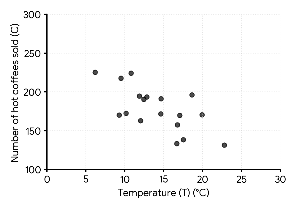
The mean temperature for these days was 15 °C.
For these results, the equation of the regression line of on is .
(a) Find the mean number of hot coffees sold.
(b) Draw the regression line on the scatter diagram.
(c) By placing a tick (✔) in the correct box, determine which of the following statements is true.
| Statement | Checkbox |
|---|---|
| The correlation is positive | |
| The correlation is negative | |
| There is no correlation |
(d) Give a reason why the regression line should not be used to estimate the number of hot coffees sold when the average temperature is 35 °C.
The regression line always passes through the point of mean values, . You are given the mean temperature, , and the equation of the line.
To draw a straight line, you need two points. You found one point in part (a), which is the point of means. The equation of the line can give you another point, for example, the y-intercept.
Observe the general trend of the data points on the scatter diagram. As the temperature increases, what happens to the number of coffees sold?
Compare the value of 35 °C to the range of temperatures for which data was collected, as shown on the scatter diagram.
Question 5
MediumPaper 1 · no calculator7 marksA biologist is studying a species of fish. The length, cm, and weight, g, of each fish in a sample are recorded.
The lengths of the fish are summarized in the following box and whisker diagram.
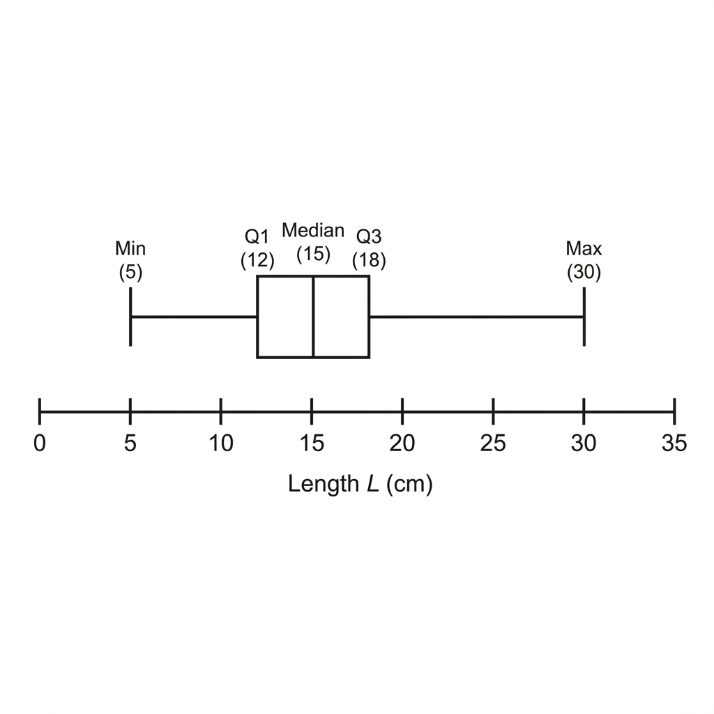
Find the largest value of that would not be considered an outlier.
The regression line of on is . The regression line of on is .
One of the fish in the sample weighs 200 g. Estimate the length of this fish.
Find the mean weight of the fish in the sample.
An outlier is defined as a data point that is more than 1.5 times the interquartile range (IQR) above the upper quartile or below the lower quartile. First, calculate the IQR.
You are given the weight () and asked to estimate the length (). You should use the regression line that predicts from .
The point , representing the mean length and mean weight, is the intersection point of the two regression lines.
Question 6
HardPaper 1 · no calculator14 marksA marine biologist is studying a species of sea turtle. She collects data on the carapace length, cm, and mass, kg, for 30 turtles. The Pearson's product-moment correlation coefficient for this data is found to be . The equation of the regression line of on is .
The biologist discovers her measuring tape was misaligned, and all length measurements are 2 cm too short. Her weighing scale was also faulty, showing a mass 1.5 kg less than the true mass for each turtle. The data is corrected for these errors.
(i) State the new value of the Pearson's product-moment correlation coefficient, .
(ii) State the new value for the gradient of the regression line of on .
(iii) Briefly justify your answers to part (a)(i) and (a)(ii).
The biologist decides to present her findings to an international conference and converts her original measurements to different units. She converts the original length measurements from cm to mm, and the original mass measurements from kg to g.
(i) State the new value of .
(ii) Find the new value for the gradient of the regression line of mass on length.
(iii) Briefly justify your answer for the new gradient.
For a different analysis, the biologist defines a "size index", , as . She investigates the relationship between the size index and the original mass in kg.
(i) Find the value of for the correlation between and .
(ii) Find the gradient of the regression line of on .
(iii) Describe the linear correlation between the size index and the mass .
The data is being corrected by adding a constant value to all length measurements and another constant value to all mass measurements. How does such a transformation (a translation) affect the correlation coefficient?
The gradient of the regression line is given by . How does adding a constant to all data points affect the standard deviations and ?
Consider the definitions of correlation and standard deviation. A translation shifts the entire data cloud without changing its shape, spread, or orientation.
The conversion from cm to mm and kg to g involves multiplying the data by positive constants. How does scaling by a positive constant affect the correlation coefficient?
The new measurements are and . The gradient is affected by the scaling of both variables. Use the formula .
Explain how the scaling of each variable affects their respective standard deviations and, consequently, the gradient of the regression line using the formula .
The new variable is . This is a linear transformation of . How does multiplying a variable by a negative number affect the correlation coefficient?
The gradient is . You have the new from part (c)(i). How does the transformation affect the standard deviation of the x-variable?
The description should include both the strength and the direction of the correlation, based on the value of you found in (c)(i).
Question 7
MediumPaper 1 · no calculator7 marksA study was conducted to investigate the relationship between the number of hours, , a student spends studying for an exam and their score, (%), in that exam.
The number of hours spent studying is summarized in the following box and whisker diagram.
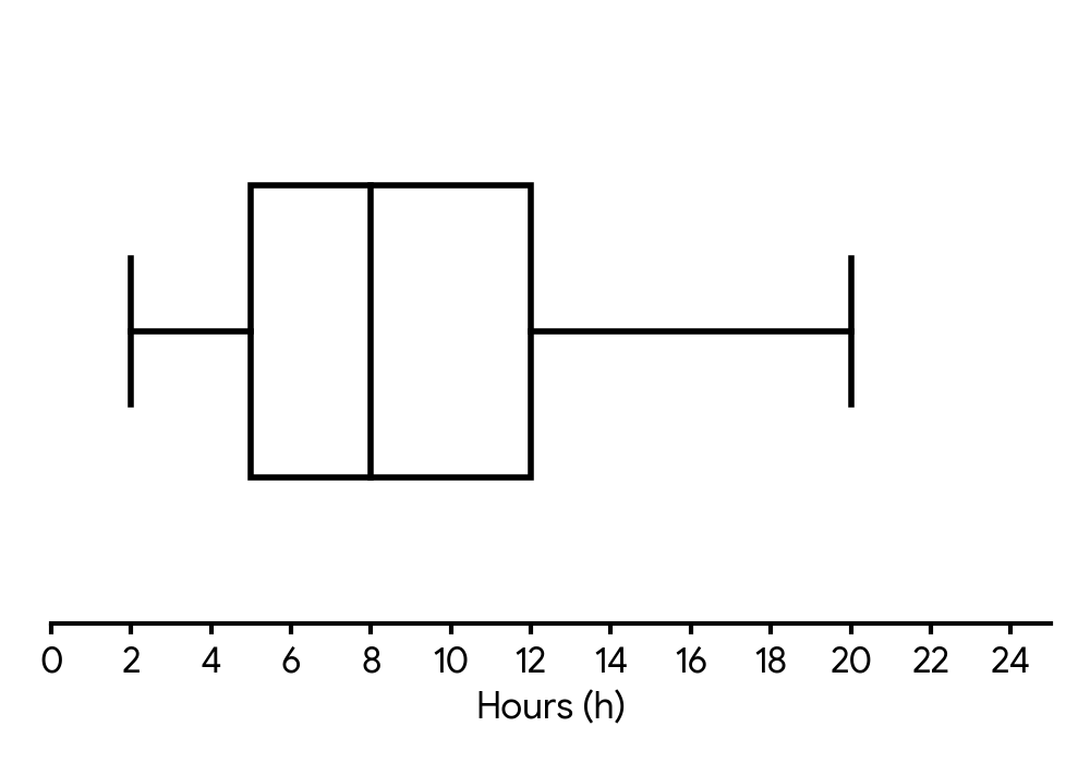
(a) Find the largest value of that would not be considered an outlier.
The regression line of on is . The regression line of on is .
(b) (i) One of the students scored 90% on the exam. Estimate the number of hours they studied.
(ii) Find the mean score of all the students in the study.
Recall the formula for identifying outliers using the interquartile range (IQR). The upper boundary is calculated as .
You are given the exam score () and asked to estimate the hours studied (). You should use the regression line of on .
The point representing the mean hours and mean score lies on both regression lines. You need to find the intersection point of the two lines.
Question 8
MediumPaper 2 · calculator7 marksA tutor wants to investigate the relationship between the number of hours a student spends studying for a mathematics test and the score they achieve on the test. They collect data from five students:
| Number of hours studied () | 2 | 5 | 7 | 4 | 8 |
|---|---|---|---|---|---|
| Test score () | 55 | 70 | 85 | 65 | 90 |
The relationship between and can be modelled by the regression line of on with equation .
Find the value of and the value of .
Write down the value of Pearson's product-moment correlation coefficient, .
Interpret, in context, the value of found in part (a)(i).
Another student studies for 6 hours for the mathematics test.
Use the regression line from part (a)(i) to estimate this student's test score.
Use your GDC's statistics function to perform linear regression (LinReg(ax+b) ). Input the values into List 1 and the values into List 2.
The Pearson's product-moment correlation coefficient () is usually calculated by your GDC at the same time as the regression line.
The value of represents the change in for every unit increase in . Consider what and represent in this problem.
Substitute the given number of hours () into the regression equation you found in part (a)(i).
Question 9
MediumPaper 2 · calculator5 marksA university lecturer is investigating the relationship between the number of hours, , students spend studying for a particular module each week and their final exam score, , out of 120. The results for eight randomly selected students are summarized in the table below.
| Study Hours ( ) | 5 | 7 | 8 | 10 | 12 | 14 | 15 | 17 |
|---|---|---|---|---|---|---|---|---|
| Exam Score ( ) | 60 | 68 | 75 | 82 | 88 | 95 | 98 | 105 |
(a) Find Pearson's product-moment correlation coefficient, , for these data.
(b) The relationship between the variables can be modelled by the regression equation . Write down the value of and the value of .
(c) One student, who currently studies 10 hours per week, decides to increase their study time by an extra three hours per week. Based on the given data, determine by how many marks their final exam score could be expected to change.
Use your GDC's statistics functions to calculate Pearson's . Input the study hours as your independent variable and exam scores as your dependent variable.
Use your GDC's linear regression function (e.g., LinReg(ax+b) or LinReg(a+bx) ) to find the values of and . Pay attention to which variable is the slope and which is the y-intercept.
The coefficient in the regression equation represents the change in for every one-unit increase in .
Question 10
MediumPaper 2 · calculator7 marksA tech company, "InnovateTech", is investigating the relationship between the average weekly training hours of its software developers and their quarterly productivity scores (out of 150). A sample of eight developers' data is collected and summarized in the table below.
| Average weekly training hours (h) | Productivity Score (P) |
|---|---|
| 12 | 82 |
| 18 | 94 |
| 25 | 116 |
| 30 | 133 |
| 15 | 86 |
| 22 | 104 |
| 35 | 145 |
| 28 | 124 |
Find Pearson's product-moment correlation coefficient, , for these data.
The relationship between the variables can be modelled by the regression equation . Write down the value of and the value of .
InnovateTech is considering providing an optional advanced training module. Based on the given data, determine how a developer's productivity score could be expected to alter if they completed this module, which adds an extra five hours of training per week.
The CEO of InnovateTech asserts that increased training hours directly cause higher productivity scores. Comment on the validity of the CEO's assertion.
InnovateTech later discovered that due to a data entry error, all recorded productivity scores were exactly 10 points lower than their true values. The data was corrected by adding 10 points to each developer's productivity score.
State how, if at all, the value of would be affected.
Use your GDC to enter the data into two lists and calculate the linear regression statistics. Pearson's is one of the outputs.
The values for and are also outputs from your GDC's linear regression calculation. Remember to round to 3 significant figures.
Consider what the coefficient in the regression equation represents. How does a change in affect ?
Think about the fundamental difference between correlation and causation in statistics. Does a strong correlation automatically imply one variable causes the other?
Consider how adding a constant to all values of one variable affects the spread and relative positions of the data points, and thus the correlation coefficient.
Question 11
MediumPaper 2 · calculator7 marksThe total number of units produced, , by a factory depends on the number of hours, , the factory operates. A production manager uses the model to predict the total units produced on any given day, where .
An energy auditor investigates the relationship between the total units produced and the energy consumption, , in kilowatt-hours (kWh). The following table shows the data collected on five different days.
Use the production model to estimate the number of units produced when the factory operates for 15 hours.
Find an appropriate regression equation that will allow the auditor to predict the energy consumption on a day when units are produced.
Hence, use your regression equation to predict the energy consumption when the factory operates for 15 hours.
Substitute the given number of hours into the quadratic model for production.
Determine which variable is the independent variable () and which is the dependent variable () for the regression. Use your GDC to find the linear regression equation.
Take the number of units produced from part (a) and substitute it into the regression equation found in part (b).
Question 12
MediumPaper 2 · calculator4 marksA marketing analyst is investigating the relationship between the amount spent on online advertising and the number of product units sold.
The following table shows the advertising spend, (in thousands of dollars), and the corresponding number of units sold, (in hundreds), for a new product over seven different campaigns.
| Advertising Spend (, in thousands of dollars) | 1 | 3 | 7 | 10 | 15 | 18 | 20 |
|---|---|---|---|---|---|---|---|
| Units Sold (, in hundreds) | 55 | 85 | 150 | 215 | 310 | 360 | 395 |
The value of Pearson's product-moment correlation coefficient, , for this data is , correct to three significant figures.
The regression line of on for this data can be written in the form .
Find the value of and the value of .
Use your regression line to estimate the number of units sold when the advertising spend is thousand dollars.
Use your GDC to perform linear regression on the given data. Input the advertising spend as your independent variable () and the units sold as your dependent variable (). The calculator will provide the values for and for the regression line . Remember to round your answers to three significant figures.
Substitute the given advertising spend value into the regression equation you found in part (a). Make sure to use the unrounded values of and for the calculation, and then round your final answer to an appropriate number of significant figures.
Question 13
MediumPaper 2 · calculator8 marksA botanist is investigating the effect of a new plant nutrient on the yield of a specific fruit crop. They apply varying amounts of the nutrient to several plants and record the amount of nutrient applied ( grams per plant) and the resulting fruit yield ( kg per plant). The results are shown in the table below.
| Amount of nutrient ( grams) | Fruit yield ( kg) |
|---|---|
The botanist wants to model the relationship between the amount of nutrient and the fruit yield using a linear regression. Find the equation of the regression line of on .
Use your equation from part (a) to estimate the fruit yield for a plant that received grams of the nutrient.
Write down the correlation coefficient .
Using the value of , describe the correlation between the amount of nutrient and the fruit yield.
Use your GDC to perform a linear regression calculation. The general form of the regression line is . Make sure to identify the values for (slope) and (y-intercept) correctly.
Substitute the given value of into the regression equation you found in part (a) and calculate the corresponding value.
The correlation coefficient is typically provided as part of the output when performing linear regression on a GDC.
Consider both the sign and the magnitude of the correlation coefficient . A value close to 1 indicates a strong positive linear correlation, while a value close to -1 indicates a strong negative linear correlation. A value close to 0 indicates a weak or no linear correlation.
Question 14
MediumPaper 2 · calculator11 marksA marketing firm analyzes the relationship between advertising expenditure and monthly product sales. They find that the sales, (in thousands of units), are strongly correlated with the advertising expenditure, (in thousands of dollars). The line of best fit for on is of the form .
When the advertising expenditure is thousand dollars, the estimated sales are thousand units.
When the advertising expenditure is thousand dollars, the estimated sales are thousand units.
Find the values of:
i
ii .
State if there is positive or negative correlation.
The marketing firm plans an advertising expenditure of thousand dollars. Find the estimated monthly sales, .
When the advertising expenditure is thousand dollars, find an estimate for the value of , given that this is an interpolation.
The gradient of a line passing through two points and is given by the formula . Apply this to the given advertising expenditure and sales data.
Once you have the gradient , use one of the given points and the equation to solve for .
Consider the sign of the gradient . If , what does that imply about the relationship between and ?
Use the equation of the line of best fit, , with the values of and you found, and substitute .
Interpolation means estimating a value within the range of the observed data. Use the same line of best fit equation.
Question 15
MediumPaper 2 · calculator16 marksA teacher wants to investigate the relationship between students' performance in Mathematics and Physics. They collect the final exam scores (out of 100) for 10 randomly selected students. The bivariate data obtained is given in the table below.
Student | | | | | | | | | |
---|---|---|---|---|---|---|---|---|---|---
Math score () | | | | | | | | | |
Physics score () | | | | | | | | | |
(a) Find the Pearson product moment correlation coefficient, , for this data.
(b) State, in two words, a description for this linear correlation.
(c) Find the equation of the line of best fit for:
i The Physics score () on the Math score ().
ii The Math score () on the Physics score ().
(d) Another student scored in Mathematics but was unable to take the Physics exam. Estimate the score they would have obtained in Physics, giving your answer to the nearest integer.
(e) A different student scored in Physics but did not take the Mathematics exam. Estimate the score they would have obtained in Mathematics, giving your answer to the nearest integer.
(f) If a student scored in Mathematics, explain why it would be unreliable to use a line of best fit to estimate their Physics score.
Use your GDC to calculate the Pearson product moment correlation coefficient. Ensure you input the data correctly into two lists or columns.
Consider the value of obtained in part (a). How close is it to or ? What does the sign indicate?
Use your GDC's regression function (e.g., LinReg(ax+b) ) with Math scores as the independent variable () and Physics scores as the dependent variable (). The equation will be in the form .
Use your GDC's regression function (e.g., LinReg(ax+b) ) but this time, set Physics scores as the independent variable () and Math scores as the dependent variable (). The equation will be in the form .
Which regression line should you use to estimate a Physics score (y) given a Math score (x)? Substitute the given Math score into the appropriate equation.
Which regression line should you use to estimate a Math score (x) given a Physics score (y)? Substitute the given Physics score into the appropriate equation.
Consider the range of the original data for Math scores. What happens when you try to predict a value far outside this range?
Question 16
MediumPaper 1 · no calculator16 marksA researcher investigates the relationship between the number of hours spent studying per week, , and the score on a standardized test, , for a group of 40 students. The Pearson product-moment correlation coefficient is found to be , and the line of best fit for on is given by .
The researcher decides to adjust the data. The number of study hours for each student is reduced by 1, and the test score for each student is increased by 5.
(a) (i) State the new value of for the adjusted data.
(ii) State the new value for the gradient of the on line of best fit.
(iii) Give a reason for your answers to (i) and (ii).
(iv) Describe in two words the linear correlation that exists for this new data.
The original data, with and , is now converted to different units. The study hours are converted from hours to minutes, and the test scores are scaled by a factor of 1.5.
(b) (i) State the new value of .
(ii) Find the new value for the gradient of the line of best fit of the scaled scores on the scaled hours.
(iii) Give a reason for your answers to (i) and (ii).
Using the original data again ( and ), a new variable called 'study deficit', , is defined as . The relationship between and is investigated.
(c) (i) State the new value of for and .
(ii) Find the new line of best fit for on .
(iii) Give a reason for your answers to (i) and (ii).
(iv) Describe in two words the linear correlation that exists for the new data.
How does adding or subtracting a constant value from all data points (a translation) affect the spread and relative positions of the points? Does this change the strength or direction of the linear relationship?
Consider the new variables and . Substitute the original equation into the expression for and then express in terms of . What is the coefficient of ?
Explain the general properties of the correlation coefficient and the regression line gradient with respect to linear transformations of the form and .
The description of correlation depends on the sign and magnitude of . What does a value of indicate?
How does multiplying all data points in a set by a positive constant (a scaling) affect the correlation coefficient?
Let the new variables be and . Use the original regression equation to find a relationship between and . You will need to substitute expressions for and in terms of and .
For , consider if scaling changes the relationship's strength or direction. For the gradient, consider how the formula is affected when and are scaled.
The transformation is . How does multiplying one of the variables by a negative number affect the correlation coefficient?
From the new variable definition, express in terms of . Then substitute this expression for into the original regression equation .
For , explain the effect of reflecting one axis. For the regression line, explain how the substitution leads to the new equation and gradient.
The description of correlation depends on the sign and magnitude of the new value you found.
Question 17
MediumPaper 2 · calculator9 marksA fitness researcher collected data on the average number of hours an individual spends exercising per week () and their average weekly calorie expenditure (, in hundreds of calories). The results for a sample of individuals are shown in the table below.
| Hours Exercised () | Calories Burned (, in hundreds) |
|---|---|
This data can be modelled by the regression line with equation .
Write down the values of and of .
Explain what the gradient, , represents in this context.
Use the model to estimate the average weekly calories burned if an individual exercises for hours per week.
Explain why it would be unreliable to use this model to predict the calories burned for someone exercising hours per week.
Use your GDC to perform a linear regression on the given data. Input the values into List 1 and the values into List 2, then use the linear regression function (e.g., LinReg(ax+b) ).
Consider the units of and . The gradient represents the change in for a unit change in . Remember that is in hundreds of calories.
Substitute the given number of hours () into your regression equation and calculate the corresponding value. Remember to convert back to total calories.
Consider the range of the values in the original data set and how hours compares to this range.
Question 18
MediumPaper 2 · calculator8 marksA research team is studying the relationship between the average daily temperature ( in ) during a growing season and the average height of a specific plant species ( in cm) at harvest. They collected data over seven growing seasons.
| Average Daily Temperature ( in ) | Plant Height ( in cm) |
|---|---|
(a) Write down the equation of the on regression line for this data, giving your coefficients to three significant figures.
(b) Estimate the average plant height if the average daily temperature during the growing season was .
Give your answer to one decimal place.
(c) The average daily temperatures were converted from Celsius to Fahrenheit using the formula .
For each of the following quantities, state whether it would change or remain the same:
(i) the mean of the average daily temperatures
(ii) the standard deviation of the average daily temperatures
(iii) the correlation coefficient,
Use your GDC to find the equation of the least squares regression line in the form . Make sure to round the coefficients to three significant figures.
Substitute the given temperature into your regression equation from part (a) and calculate the corresponding plant height. Remember to round to one decimal place.
Consider how adding a constant and multiplying by a constant affect the mean of a dataset.
Consider how adding a constant and multiplying by a constant affect the spread (standard deviation) of a dataset.
Think about whether a linear transformation affects the strength and direction of the linear relationship between two variables.
Question 19
MediumPaper 2 · calculator8 marksA local coffee shop records its weekly sales of two popular coffee beans, Espresso Blend and Single Origin, over 10 weeks. The sales figures, in kilograms (kg), are shown in the following table.
Weekly Sales (kg)
| Cafe Week | 1 | 2 | 3 | 4 | 5 | 6 | 7 | 8 | 9 | 10 |
|---|---|---|---|---|---|---|---|---|---|---|
| Espresso Blend () | 50 | 65 | 70 | 55 | 80 | 75 | 60 | 90 | 85 | 95 |
| Single Origin () | 57 | 66 | 74 | 67 | 78 | 74 | 71 | 91 | 81 | 94 |
The cafe manager determines that the equation of the regression line of on for these sales is .
Find the value of Pearson's product-moment correlation coefficient, .
The new cafe manager uses the regression line of on () for making predictions.
One week, Espresso Blend sales were kg. The manager estimated Single Origin sales to be kg. Give a reason why this estimation might not be appropriate.
Another week, Single Origin sales were kg. The manager used the line to estimate Espresso Blend sales as kg. Give a reason why this method is not appropriate.
Use an appropriate method to show that the estimated Espresso Blend sales for the week when Single Origin sales were kg is kg (to the nearest integer).
Use your GDC to calculate Pearson's product-moment correlation coefficient () for the given bivariate data. Remember to input the values as the independent variable and values as the dependent variable.
Consider the range of the original data for Espresso Blend sales (). Is kg within this range?
Think about which variable is being predicted and which regression line is appropriate for that prediction.
You need to find the equation of the regression line of on and then use it to predict when .
Question 20
MediumPaper 2 · calculator4 marksA group of six students recorded the number of hours they spent studying for a mathematics exam, , and their corresponding score on the exam, , out of 100.
The data is presented in the table below:
| Weekly Study Hours () | Exam Score () |
|---|---|
| 8 | 60 |
| 10 | 68 |
| 12 | 75 |
| 14 | 82 |
| 16 | 88 |
| 18 | 95 |
The regression line of on for this data can be written in the form .
Find the value of and the value of . Give your answers to three significant figures.
Use the equation of the regression line to estimate the exam score of a student who studies for hours per week.
Use your GDC's regression function (e.g., LinReg(ax+b) ) to find the values of and . Remember to input the values into one list and the values into another.
Substitute the given number of study hours into the regression equation you found in part (a) to estimate the exam score.
No question on this page matches those filters. Try another difficulty or paper.
3 more Regression lines and reverse regression (x on y) + applications questions in the app
Every answer is marked mark by mark, IB-style, and the AI tutor helps when you are stuck.
Where marks are lost
- Rounding an intermediate value and then using it.
- Answering to the wrong accuracy. Two significant figures, or six, where the rule says exactly or three.
- Writing the answer and nothing else.